News — 30 August, 2019

Using Open Source Tools to Solve Routing Issues for Solid Waste Collection in Dar Es Salaam

One of the biggest difficulties in establishing an effective and efficient waste management collection and transportation system in Dar es Salaam is how long it takes to travel to Pugu dumpsite, the only officially designated solid waste dump in the city, and the best route to use.

Depending on the time of day, it can take up to five or more hours for a return trip from certain points in the city. If there is a designated route for those collecting trash and taking it to the main dumping site, it will increase efficiency and planning for solid waste collectors and improve the quality and reliability of solid waste collection in the city.

An informal solid waste dump site in Dar es Salaam. The number of sites like these could be greatly reduced with better collection planning and scheduling.

Choosing the best way to get from A to B – also known as routing – is an essential part of many mapping platforms and the feature that most people use maps for every day. Think about it – GoogleMaps, Waze, MapQuest, Bing, the list goes on. Yet amid this flourishing routing ecosystem, open-source tools and OpenStreetMap have lagged behind in routing capabilities. Now, the tools to creating better open-source routing tools are at our fingertips!

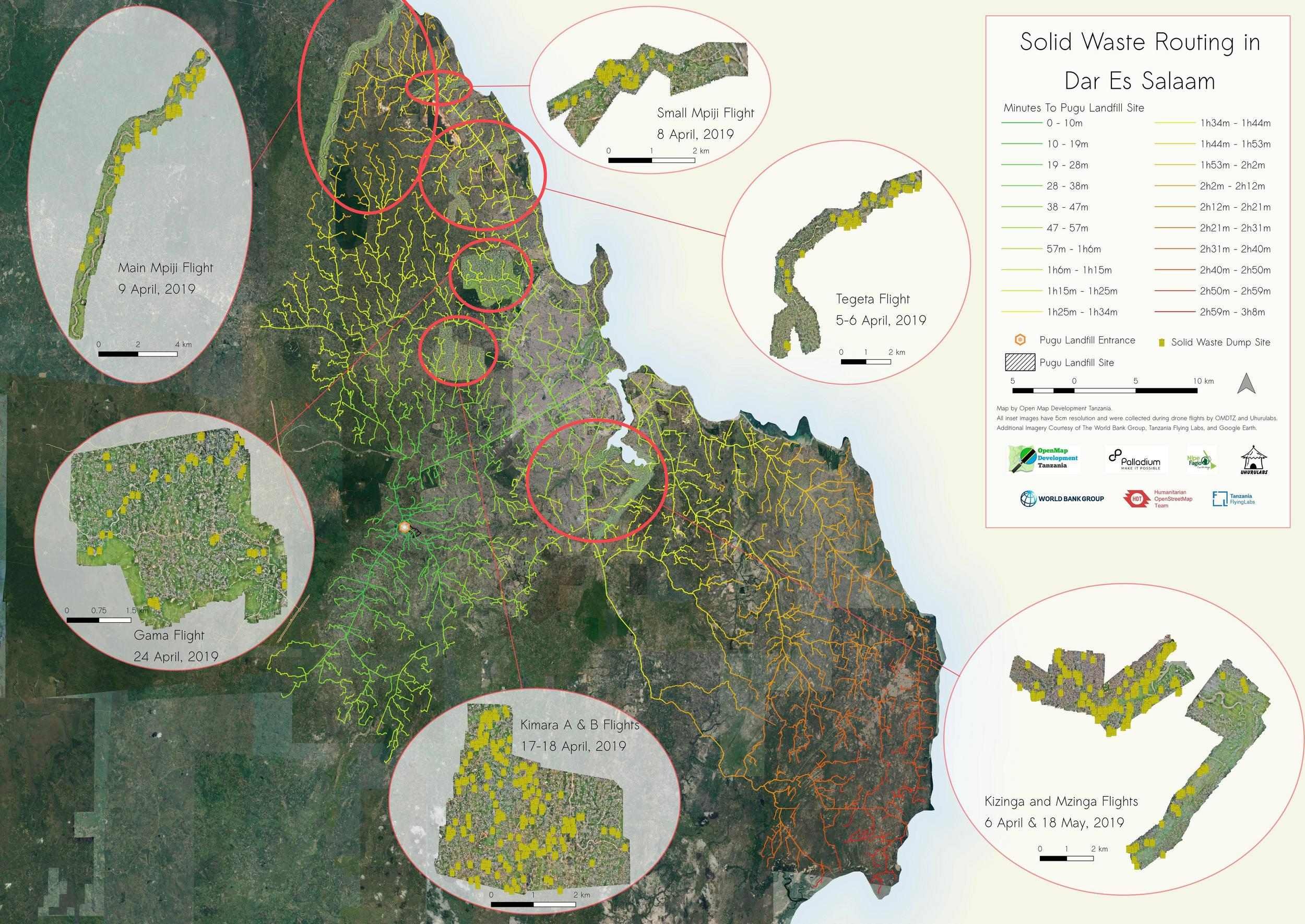
As part of a project funded by Palladium and I4ID to map solid waste near rivers in Dar Es Salaam, the HOT Tanzania team has developed a routing scheme for the city using pgRouting, an open-source extension to the PostgreSQL database management system. The aim of this project was to create a routing system to understand how long it would take to travel from sample points throughout the city to the Pugu Kinyamwezi Landfill located in Southwest Dar Es Salaam (see map below). This would then help trash collection companies, sanitation officials, and government planners more efficiently prepare routes for collection of solid waste.

The Pugu Kinyamwezi dumpsite.

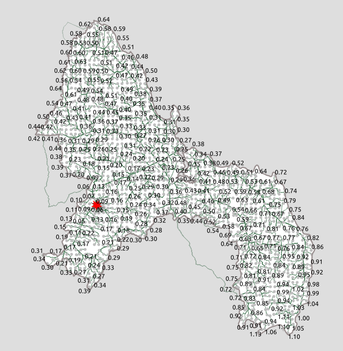
The results were astounding. With a few lines of SQL, we were able to create routes from nearly 1,500 sample points in the city in less than five seconds of processing. Using Djikstra’s shortest path algorithm with a weighting scheme that assigned a higher cost to roads we know to be more difficult to traverse. For example, residential and unclassified roads, which are most often unpaved and very slow to traverse in Dar Es Salaam, may have a cost of 5 or 6, while the main trunk road (a primary highway) and a secondary highway (which are almost all paved in Dar) would have a cost of 1.1, 1.2, and 1.3 respectively. Thus, when we make a route from one point to another in our network dataset, we are not just getting the shortest distance from point A to point B, but the route is actually taking us on the most logical path through the line segments based on the weights that we have assigned. In the figure below, you can see a comparison of routes with different weights.

The route in red shows the shortest distance route, while the magenta adds in a high-cost multiplier to low-level roads (residential, single-lane unpaved), and the orange builds in a fully weighted scheme where the highest order roads are given the most preference.

The type of road isn’t the only consideration when considering a routing problem. There are plenty of real-world issues like traffic (which is particularly bad in Dar es Salaam), road surface type, elevation, speed limits, and if vehicles (in this case, a large standard garbage truck) can navigate the roads. Roads susceptible to flooding would also not be preferable. With pgRouting (and some rigorous data collection) you can incorporate all of this data into your schema to give an exceptionally accurate model of routes – and even travel times – in a city.

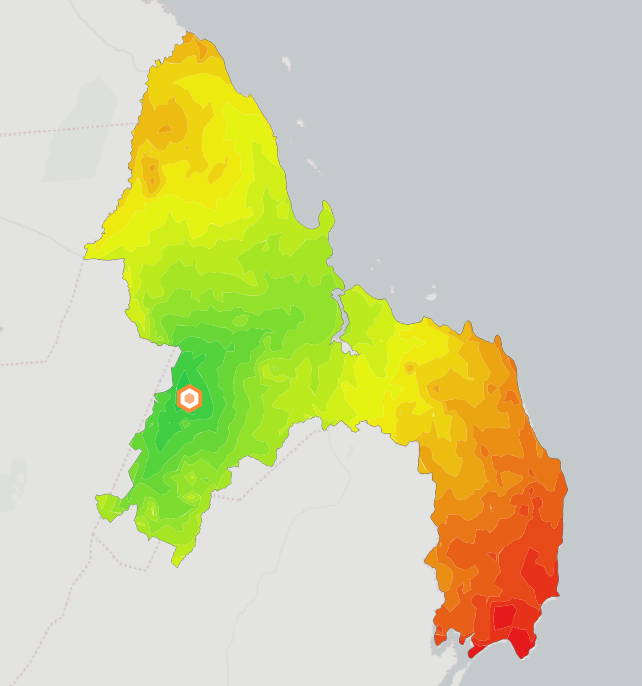
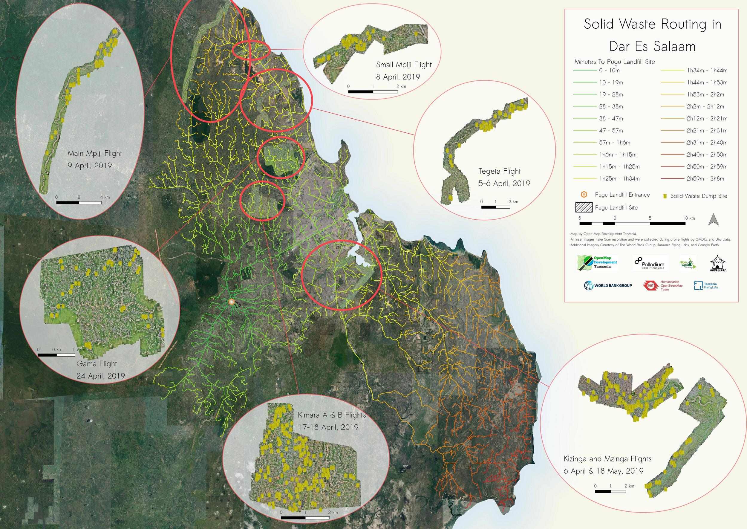
With our routing model, we layered a time-approximation scheme on top of our arbitrary cost outputs to generate travel times (in minutes) from every sample point to the Pugu landfill. We then visualized these times with isochrones in QGIS and pared them down to just the road segments, highlighting the accessibility to Pugu from any point in the city (see map below). We also took solid waste sites digitized from drone imagery collected during the project to visualize the efforts necessary to collect the solid waste collected near rivers, which are particularly problematic spots for informal dumping.

Routes from sample points in Dar Es Salaam to the Pugu dumpsite, with color change representing time to the site. See how to make this below!

The possibilities for routing don’t stop at solid waste collection. pgRouting could be used for any number of applications including bus routing, fleet deployment for businesses and delivery services, aid logistics, and resource allocation for hospitals and local health clinics, just to name a few. The use of Postgres also allows these tools to be highly adaptable to many applications, meaning the tools can be directly embedded into your next application — without the use of an API or a third-party software.

Below, you’ll find the steps to create your own pgRouting network dataset and see how to create routes from node to node in your network. Note that this tutorial takes you through the steps primarily using Linux (which you should be using), which we have extensively tested. We did our best to give accurate instructions for other operating systems, but there may be differences for Mac and Windows users.

Please contact us at omdtanzania@gmail.com or eubank.aaron@gmail.com if you find our information could be improved in any way.

Step-By-Step Tutorial: Routing in Dar Es Salaam

1. Prereqs: Install PostgreSQL and PostGIS

PostgreSQL and its PostGIS extension are prerequisites for running pgRouting, so make sure these are installed on your system first. This post for Linux and this video for Windows can help get you started.

Additionally, you’ll want to have the latest version of QGIS downloaded, which is not only great for visualization, but also serves as your *PostgreSQL*administrator, allowing you to run your queries directly from the QGIS database manager (in fact, QGIS started because its creator, Gary Sherman, wanted a way to easily view his PostGIS data on his home Linux machine, so the QGIS-Postgres connectivity is exceptionally mature).

Windows users will want to download and install the PostGIS bundle with the StackBuilder application that ships with PostgreSQL (or ensure that the PostGIS bundle for PostgreSQL 11 option is checked when initially downloading PostgreSQL). This will also install pgRouting, so you can skip step 2.

2. Install pgRouting

For Linux users, pgRouting can be installed by following the instructions here.
Mac users using homebrew can find pgRouting using this command:

brew install pgrouting
Windows users, install using the PostGIS bundle installation detailed in step 1.

3. Create Extensions for PostGIS and pgRouting

Use the following query within the Postgres database of your choice to create the necessary extensions to use pgRouting:

                      `   `*` CREATE EXTENSION PostGIS;

CREATE EXTENSION pgrouting;`* If you’re using pgAdmin4 to do this, you should see this when you click on the extensions for your database:

4. Download your roads dataset from OSM using the HOT Export Tool

Follow the instructions on the HOT Export Tool to choose your area of interest and download the data as an OSM *.pbf * file.

Note: if you wanted to consolidate steps 4 and 5, you can also download .osm data directly from the site using Overpass Turbo.

5. Convert your .pbf file to a .osm XML file for use with osm2pgrouting using osmconvert

OSM* XML* files (using the* .osm* extension) are required for the osm2pgrouting tool and the HOT Export Tool does not support* .osm* downloads. So you’ll need to convert your .pbf file to .osm using osmconvert.

To install on Linux:

sudo apt install osmctools

Windows binaries can be downloaded here.
The tool doesn’t seem to be compatible with Mac, so try using Overpass (see above).
Enter the following command in the Terminal/Command Prompt to convert:

osmconvert path/to/file/yourfile.pbf > yourfile.osm

6. Use osm2pgrouting to Create Your Network Dataset

To install osm2pgrouting on Linux:

sudo apt-get install osm2pgsql

Here are instructions for Mac download.
For Windows, this conveniently comes as part of the PostGIS Bundle. If you followed step 1, you should already have osm2pgrouting!
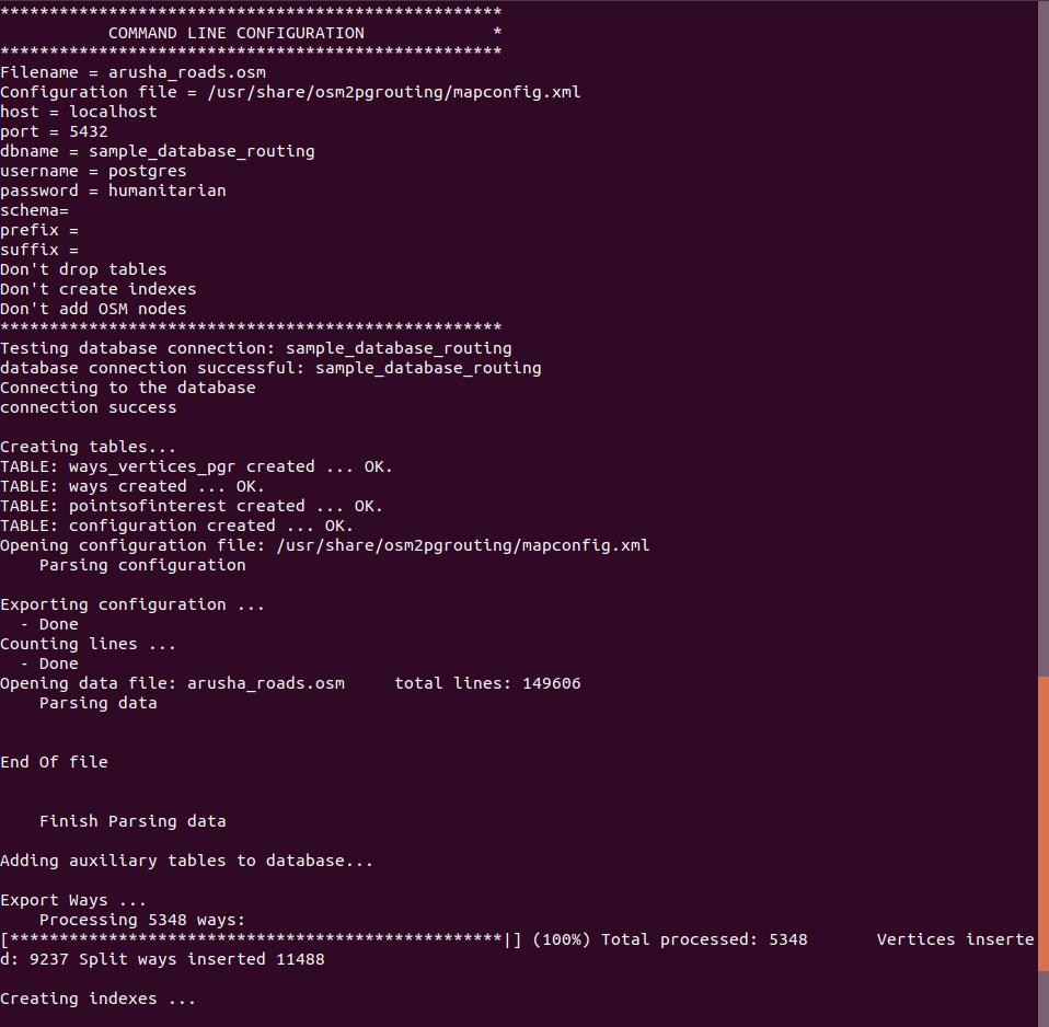
Once you’ve downloaded, here is the command to create a new network dataset in the Terminal/Control Panel:

sudo osm2pgrouting -f your_filename.osm --dbname yourdb_name -U your_user -W your_user_password

#drop the "sudo" in Windows & Mac

Your output should look something like this:

Note: You can also manually create a network dataset using only pgRouting and your data. More on how to do that here.

7. Set up your Postgres database in QGIS

This process will allow you to quickly and easily visualize any queries that you run with Postgres. As mentioned above, QGIS will also serve as your administrator for Postgres, where you can run your queries and manage your database. For instructions on how to connect to your Postgres database, check out this post.

Once your connection is set up, head on over to the DB Manager to access your database.

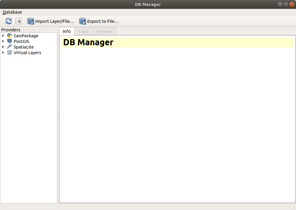
The DB Manager links directly to your Postgres server and is a surprisingly sussed out admin tool. It is where we ran most of our queries and has some wonderful features including the ability to turn your queries directly into QGIS layers.

To access the SQL Window to run SQL queries, click this icon:

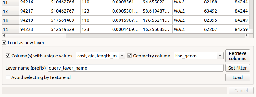
To save a query as a layer, run the query, then click the “Load as new layer” box at the bottom, fill out the details, then click “Load” to see your layer in the QGIS canvas. This is the best way to visualize your queries going forward.

With the DB Manager, you are also able to easily save your SQL queries within your QGIS project by giving a name to your query and clicking “Save” at the top of the query dialogue.

8. Understanding Your Data Tables

pgRouting creates several data tables for your network dataset, but the most important will be the ways table (the lines for your roads, the *ways_vertices_pgr *table (the connecting nodes for all of the lines in your dataset) and the *configuration *table (which gives you information about the type of road in the ways table).

Here is a look at each of the tables and what their important attributes mean:

The ways Table:

This is a table of all of the individual line segments of your dataset. Some important fields here include:

tag_id: gives the type of road for the line segment (reference the configurationtable).
length: represents the length in degrees of the line segment.
length_m: represents the length in meters of the line segment.
source: the starting node of the line segment in reference to the idfield of the ways_vertices_pgr table.
target: the ending node of the line segment in reference to the id field of the ways_vertices_pgr table.
cost: gives the cost necessary to move across the linestring for routing purposes. By default, this represents the length (in degrees) of the line segment.
cost_s: represents the cost with speed of the road taken into account. For our dataset, speed was the same for every line segment (a default of ‘50’), so this was not a meaningful metric (but could be with accurate speed data).
reverse_cost & reverse_cost_s: the cost to go the opposite direction over the linesegment. This would come into play if you added something like elevation to your network dataset when you were compiling it.

The ways_vertices_pgr Table:

This table contains all of the connecting nodes of line segments in your dataset. The important field here is:

id: the reference number for the node that will allow you to choose it as the starting point for routes and is used as a reference in the ways table.
The configurationTable:

This is derived from your input XML file that we converted in step 5. It contains important information for interpreting your ways table. The most important fields are:

tag_id: corresponds with the tag_id in the ways table and gives information on the type of way.
tag_key: lets us know the key of way tag (i.e. road or cycleway).
tag_value: lets us know the specific class of road.

9. Creating a Weighting Schema

The default cost output in your ways table will be the same as the distance (in degrees). If you look carefully at the table, the distance (in degrees) column has the same value as the cost, indicating that distance is the only thing affecting cost. We want to change that up to better reflect the cost to travel on our roads. There are many ways you can do this, but here is what we did to create a weighting based on the type of road:

Look up the tag_id values in the configuration table (see step 8 above) so that you can determine what tag the values correspond to.
Create a new column in the ways table that groups the roads by type of road that you would like to use.

Here’s how our query looked:

ALTER TABLE ways ADD road_rank bigint;

UPDATE ways
SET road_rank = 1
WHERE tag_id = 104 or tag_id = 105; --trunk roads

UPDATE ways
SET road_rank = 2 WHERE tag_id = 106 or tag_id = 107; --primary roads

UPDATE ways
SET road_rank = 3 WHERE tag_id = 108 or tag_id = 124; --secondary roads

UPDATE ways
SET road_rank = 4 WHERE tag_id = 109 or tag_id = 125; --tertiary roads

UPDATE ways
SET road_rank = 5 WHERE tag_id = 110 or tag_id = 112 or tag_id = 113 or tag_id = 123; --unclassified, track, residential and service roads

UPDATE ways
SET road_rank = 6 WHERE tag_id = 117 or tag_id = 114 or tag_id = 119; --footpaths, paths, or footways

--We then deleted anything that was null here (i.e., cycling paths, horse paths) because we did not want to use it in our weighting DELETE FROM ways WHERE road_rank is null;

3. Create a new cost field, weighting how you would like the roads prioritized.

Here is our final cost schema:

UPDATE ways
SET cost_4 = (1.1 * length) --nominal cost multiplier mostly for gas and wear & tear. WHERE road_rank = 1;

UPDATE ways SET cost_4 = (1.2 * length) --slightly higher for primary WHERE road_rank = 2;

UPDATE ways
SET cost_4 = (1.4 * length) --and for secondary WHERE road_rank = 3;

UPDATE ways
SET cost_4 = (1.6 * length) --and for tertiary WHERE road_rank = 4;

SET cost_4 = (3.5 * length) --considerably higher for smaller, slower, generally unpaved roads WHERE road_rank = 5;

UPDATE ways
SET cost_4 = (10 * length) --you could choose to remove footpaths altogether, but we kept them and gave them a VERY high-cost multiplier WHERE road_rank = 6;

10. Test Your Dataset With Some Routing Queries!

Your possibilities for routing are limited only by the number of ways and node in your network dataset!

pgRouting has several different routing functions, which can be read about here. We chose the pgr_dijkstra function, which gives the least-cost path between two nodes in the network dataset.

You can choose your start and endpoint for a given route by selecting these nodes in the ways_vertices_pgr table (loaded in QGIS) then determining the value in the id field within the attribute table, which will correspond with the arguments needed in your pgr_djikstra query.

Or, you can just enter random points and see what route you get!

Here are a couple of different queries to get your routes started:

Basic One-to-one Route SELECT seq, node, edge, a.cost, b.the_geom FROM pgr_dijkstra( 'SELECT gid AS id, source, target, cost_column_name AS cost FROM ways', 121157, 63711, FALSE) a LEFT JOIN ways b ON (a.edge = b.gid);

--points are examples only, use your own points from the "Source" field in your "ways" table

Many-to-one Route SELECT seq, node, edge, a.cost, b.the_geom FROM pgr_dijkstra( 'SELECT gid AS id, source, target, cost_column_name AS cost FROM ways', ARRAY[32, 234, 434, 121157], 51227, FALSE) a LEFT JOIN ways b ON (a.edge = b.gid);

--points are examples only, use your own points from the "Source" field in your "ways" table

Remember that you can save your queries as QGIS layers using the instructions in section 2.

You can also add this snippet at the beginning of your query to save the route as a PostGIS table on your Postgres server:

CREATE TABLE table_name AS SELECT seq,....

Doing More with Your Routing: Creating Sample Points to Show Fastest Routes from Various Places Around a City

a. Create sample points throughout a bounded area using grid centroids

Use the “Create grid” tool to place a grid over your area of interest. If you want it fit to a specific shapefile’s area (we used Dar Es Salaam, for example), choose “Use Layer Extent…” in the “Extent Field”. Choose a distance for your grid (we did 2km by 2km) and ensure that you have a project projection set if units other than degrees are not showing up in the dialogue box.
Use the “Centroids” tool to get the centroids of your grid layer.

b. Snap these sample points to nodes in your network dataset

In order to “snap” these points to the road layer, we’ll follow a three-step process:

Use “Distance Matrix” to get the nearest neighbour from the “ways_vertices_pgr” layer. Choose your centroids as the input, “ways_vertices_pgr” and “1” in the “Use only the nearest (k) target points”. This will return a layer with the input points and the nearest point from the vertices layer.
This new layer now has the previous point and the target point together as a single multipart feature. We need to break these apart, so first we will use the “Multipart to singleparts” tool to do so.
Next, run an intersection with the “singleparts” layer just created and the “ways_vertices_pgr” layer to yield the sample points “snapped” to your road network.

c. Save the sample points as a new table in your Postgres database

Use the DB Manager, navigate to your database and click “Import Layer/File” at the top.

Call it something like final_sample_points and click “Create Spatial Index”.

d. Run a many-to-one Dijkstra routing function, creating a route from every point in your table of sample points

Here is the query you’ll need to pull in your points from another table:

CREATE TABLE table_name AS SELECT seq, path_seq, start_vid, node, edge, a.cost, agg_cost, osm_id, b.the_geom FROM pgr_dijkstra( 'SELECT gid AS id, source, target, cost_column_name AS cost FROM ways', (SELECT ARRAY(SELECT node_field FROM final_sample_points), 51227, FALSE) a LEFT JOIN ways b ON (a.edge = b.gid);

-- if you follow the steps above, 'node_field' should be 'id_2' -- point values given are examples only, use your own routing points from the "source" field in your "ways" table

Did you see how fast that went? Save your routes as a layer and see how it looks in the QGIS canvas.

e. Visualizing aggregate cost of routes

Now that you’ve run your routes, you may want to visualize them! Here is a workflow to do that:

Coercing aggregate cost to your sample points:

If you take a look at the attribute table for your routes, you’ll see that each segment for a given route has an aggregate cost associated with it. These costs build up until they reach the maximum cost.

In order to coerce the maximum aggregate cost (and therefore the total aggregate cost) from each route into a new table, we can run the following query:

CREATE TABLE cost_join AS SELECT start_vid, agg_cost FROM route_all WHERE cost = 0.0;

This query takes every point in the attribute table where cost = 0, which is also the row where aggregate_cost is at its maximum. It throws out the extraneous information while preserving the start_vidattribute (which corresponds with the starting node of the route).
Now, we can join this table to our final_sample_pointslayer from step 11c above using the following query:

CREATE TABLE sample_points_cost AS SELECT fid, geom, id_2, osm_id, lon, lat, agg_cost FROM final_sample_points LEFT JOIN cost_join ON id_2 = start_vid --This line will be specific to your tables, but these fields should match

Now you have a new table with cost values appended to your final sample points! You can label all of the starting points with the total aggregate cost to your destination.

The next step discusses creating a contoured “heatmap” of the cost based on this data.

2. Creating a contoured “heatmap” of your aggregate cost

First, install the QGIS Contour plugin.

Before you run the tool, Contour only works with single-point data and your ‘sample_points_cost’ layer may be multipart based on the steps above. Go ahead and create a single parts layer using the ‘Multipart to singleparts’ tool and feed that output into the Contour tool.

You’ll want to use your aggregate_cost as your field to can choose as many or as few contours as you’d like, but we found that 20 was a good number. Your styled output will look something like this:

3. Joining contours with the routes only

We liked the contours but wanted them to be a little less pronounced, so we sought to show only the route lines with the contour symbology. While slightly buffering the routes, then clipping the contours to them would have been an obvious solution, this would not have given us dynamic rendering of the data at different scales (as the width of each line would be fixed).

So our solution was to spatially join the routes layer with our aggregate cost added to the cost in QGIS using the “Join attributes by Location” tool. Use the dialog box below to do so. Be sure to also use the raw contour file (before any clipping you may have done). This will ensure that all of your roads are assigned a value.

Your output should look something like this:

f. Converting aggregate cost into a more meaningful metric

As it stands, our aggregate_cost field doesn’t mean much to us, since cost here is a pretty arbitrary value based on the distance weighted by the type of road. Ideally, we’d like to get this in a format that gives us some actionable information. Travel time is an obvious option.
Because we didn’t have a tremendous amount of data on speeds of roads and traffic for Dar Es Salaam, we ended up referencing a handful of routes from a major tech company’s routing tool and applying our local knowledge of travel times (i.e. slightly informed guessing) to create a logarithmic equation to our aggregate_cost field.
Note: Lacking the ability to think of a way to do this properly, we performed a manual curve-fit (in other words, we set up a basic logarithmic expression and tweaked the parameters until our answers looked like the ones we had already calculated/guessed). Don’t try this at home. At home, actually, determine the speeds on your road network—which is what we plan to do when time permits!*
We created a new field cost_mins on our sample_points_cost layer from step 11e(1) above (make sure you add your table to Postgres to follow the step below. You could also do this in the field calculator of QGIS with different syntax), then applied the logarithmic equation in the field calculator as follows:

ALTER TABLE nodes_table_to_modify ADD cost_minutes bigint;

UPDATE nodes_table_to_modify SET cost_minutes = log(agg_cost + 1.01)*600; -- Here is the logarithmic equation we used, just an example -- Yours will likely be different -- We made ours up

This gave us a nice travel time field that we could also apply to our various visualizations above.

g. Our final data product:

12. Extra Resources and Sources Used

Resources

We have built our tools on previous work of some of the brilliant people in the free/open-source GIS community. In particular, the incredible body of work of Anita Graser (@underdarkGIS) has been helpful to us in doing this and other projects, as has Paul Ramsey’s blog.

Keep in mind that some of these resources are old, potentially outdated, or use older versions of the tools above.

Links to The Software and Extensions Mentioned In This Post (Also Linked Within)

Mapping our world together